
RapidKnowHow® ●
THE DECISION COMPANY™
POWERREPORT · BUSINESS OWNERS · CxOs · BOARDS · INVESTORS
When Should You Change Industrial Gas Supply?
Volume screens the options.
Total cash cost decides.
Change your supply model when a technically qualified alternative improves your whole-life cash outcome while meeting the required purity, pressure, capacity and reliability.
ONE JOB → ONE STRATEGY → ONE ACTION → ONE VERIFIED RESULT
1. ONE JOB: Secure the Gas Your Business Needs
Start with the customer’s production requirement—not the supplier’s preferred equipment.
- Gas: oxygen, nitrogen, argon or another specified gas.
- Quality: composition, purity and allowable impurities.
- Flow: average demand, peak demand and variability.
- Pressure: required at the point of use.
- Operating pattern: hours, shifts and seasonal changes.
- Reliability: backup capacity and acceptable interruption.
A lower price per Nm³ creates no value if the gas cannot perform the required job or if interruptions reduce production.
2. When Should You Review the Supply Model?
| Trigger | Business Question |
|---|---|
| Demand grows or declines | Does the current model still fit actual utilisation? |
| Deliveries become frequent | Are logistics and handling consuming the price advantage? |
| Rental or idle stock increases | Are you paying for capacity you no longer need? |
| Service becomes inadequate | What is the cost of shortages, pressure problems or emergency supply? |
| Contract renewal approaches | Can competing supply models improve the next contract? |
| A new supply option becomes available | Does a nearby pipeline or suitable onsite technology change the economics? |
3. Compare the Supply Options
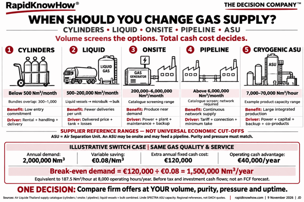
The following published supplier ranges help screen alternatives. They are regional reference ranges—not universal economic cutoffs or DACH quotations.
| Supply Model | Published Reference Range | Cash Drivers |
|---|---|---|
| Cylinders / Bundles |
Cylinders: below 500 Nm³/month. Bundles: 300–1,000 Nm³/month. |
Gas price, rental, handling, delivery and idle stock. |
| Liquid Supply |
Liquid vessels: 500–2,000 Nm³/month. Microbulk: 2,000–5,000 Nm³/month. Bulk: 5,000–200,000 Nm³/month. |
Delivered price, tank charges, site works, losses and backup. |
| Onsite Generation | 200,000–6,000,000 Nm³/month in the referenced regional catalogue. | Electricity, utilisation, plant payments, maintenance and backup. |
| Pipeline | Above 6,000,000 Nm³/month in the same catalogue. | Network availability, connection, tariff, escalation and minimum take. |
| Cryogenic ASU | Linde SPECTRA example: 7,000–70,000 Nm³/hour. This is a product capacity range. | Capital, power, maintenance, backup and supportable co-product value. |
Important: these options overlap. An ASU can be built onsite and can feed a pipeline. Pipeline describes delivery; ASU describes production. There is no mandatory five-step ladder.
Smaller onsite technologies also exist. For example, Linde lists VITRON oxygen VPSA units at 500–1,000+ Nm³/hour with oxygen purity up to 94%. The process must accept the available purity.
Nm³ measures gas volume at agreed normal reference conditions—not litres of liquid. Align reference temperature, pressure and composition across quotations. Keep monthly volume, annual volume and hourly capacity clearly separated.
4. ONE STRATEGY: Compare the Same Customer Outcome
Ask suppliers to quote the same demand profile, gas specification, pressure, reliability and evaluation period.
- Operating cash: gas, power, logistics, rental, maintenance and backup.
- Investment cash: equipment, installation, connection and replacement.
- Working capital: inventory, deposits and payment terms.
- Transition cash: temporary supply, termination, removal and commissioning.
- Contract exposure: minimum take, escalation, duration and exit obligations.
Compare customer ownership with supplier build-own-operate offers. Lower upfront investment may come with longer payment commitments.
5. Calculate the Economic Cutoff
Where the alternative has higher annual fixed cash costs but lower variable costs, use this first screening calculation:
Break-even annual demand =
Extra annual fixed cash cost ÷ Variable saving per Nm³
This assumes constant unit costs and equivalent technical performance. It does not replace a full investment appraisal.
6. Illustrative Business Case
ASSUMPTIONS — NOT SUPPLIER QUOTATIONS OR VERIFIED RESULTS
Compare existing delivered supply with a technically qualified alternative providing the same gas quality and service.
| Input / Result | Illustrative Value |
|---|---|
| Annual demand | 2,000,000 Nm³ |
| Variable saving | €0.08/Nm³ |
| Annual variable cash saving | €160,000 |
| Extra annual fixed cash cost | €120,000 |
| Annual operating cash advantage | €40,000 |
| Break-even annual demand | 1,500,000 Nm³ |
| Equivalent average operating flow at 8,000 hours/year | 187.5 Nm³/hour |
At only 1,000,000 Nm³/year, these assumptions produce a €40,000 annual operating disadvantage. A lower unit cost does not compensate for insufficient utilisation.
These results are before tax and investment cash flows. They are not complete FCF forecasts.
7. Convert the Saving into a Free Cash Flow Case
Include transition and exit costs in the relevant cash periods. Add evidenced disposal proceeds separately when received, allowing for tax where applicable. Avoid counting the same cost twice.
Compare discounted cash flows over a common evaluation horizon. Test low demand, higher electricity prices, interruptions and contractual commitments.
Calculate ROCE using consistent EBIT and average capital employed. FCF divided by opening investment is not ROCE.
8. ONE ACTION: Build ONE Site Decision Sheet
- Collect 12 months of invoices and consumption.
- Record operating hours, average flow and peak requirements.
- Confirm purity, pressure, backup and uptime requirements.
- Obtain comparable offers for the current model and feasible alternatives.
- Have operations qualify service and finance reconcile the cash case.
9. ONE VERIFIED RESULT
After the change, compare actual gas cost, energy, logistics, maintenance, backup, inventory and reliability with the approved baseline. Adjust for volume and price changes.
Separate one-time working-capital release from recurring cash improvement. Verify investment payments and net benefits against invoices and financial records.
Change supply when the whole-life cash benefit justifies the switch and the required production performance is secured.
Sources
- Air Liquide Thailand — Supply Mode catalogue : regional supply-volume reference ranges.
- Linde — On-site ASUs : integrated production and SPECTRA capacity example.
- Linde — VITRON oxygen onsite plants : small VPSA capacity, purity and backup.
Published 9 November 2026. Supplier ranges describe available options. The financial example is illustrative RapidKnowHow® analysis. No verified customer outcome is claimed.
RapidKnowHow® — Knowledge is useless unless it improves someone’s life.
© Josef David · RapidKnowHow® · rapidknowhow.com
RapidKnowHow® — THE DECISION COMPANY™
Industrial Gas Leadership 2030
PROVE VALUE. THEN SCALE.
Watch the 60-second roadmap: 10 strategic actions for DACH and CEE, 2026–2030.
Start with ONE customer challenge. Use the Industrial Gas Action Guide to turn your first action into a measurable result.
RapidKnowHow® — Leading Industrial Gas Opportunity Signal Identifier in DACH & CEE